Resampling Optimal Asset Discribution

Completeted March 2024

Technologies Used: R

I collaborated with a group of my peers to examine the viability of using bootstrap resampling to simulate portfolio returns.

We examined a hypothetical three asset portfolio (Apple, Meta, Tesla), calculating monthly returns from January 2019 to December 2023. We obtained this data from Yahoo Finance, and evalulated these assets using mean-variance analysis, which uses mean and variance/standard deviation to quantify an investor's risk-return tradeoff decision.

We calculated the following collection of asset spreads for the historical data:

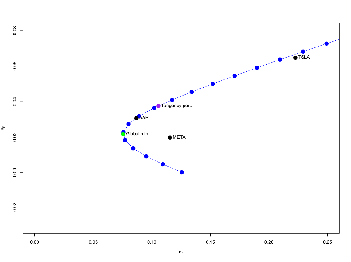
1. Global Minimum Variance Portfolio (GMVP): Spread of assets with lowest risk.
2. Efficienct Frontier (EF): Collection of Portfolios with highest return for a given risk.
3. Tangency Portfolio (TP): Most optimal spread of assets, given an alternative risk-free asset with a return of 0.5%.

GMVP, EF, TP from historical data

We then used bootstrap resampling to create 500 alternative return spreads through sampling with replacement, and examined how close those random samples reflected the original value.

I was personally responsible for implementing the bootstrap analysis for the Efficiency Frontier & Tangency Portfolio. The following code was used to perform the bootstrap resampling. I used ggplot2 to create visualizations of the simulations.

boot_tp <- function(mu, cov, rf) {
  tryCatch(
    expr = {tangency.portfolio(mu, cov, rf)},
      error = function(e) {NA})}

ef.list = list()
tp.list = list()

for (i in 1:n.boot) {
  boot.idx <- sample(n.obs, replace=TRUE)
  ret.boot <- gwnReturns[boot.idx, ]
  mu.boot <- colMeans(ret.boot)
  cov.boot <- cov(ret.boot)
  ef.list[[i]] <- efficient.frontier(mu.boot, cov.boot)
  tp.list[[i]] <- boot_tp(mu.boot, cov.boot, r.f)
}

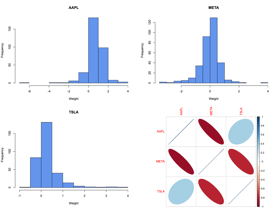
Histograms and correlation of asset spreads across calculated Tangency Portfolios.

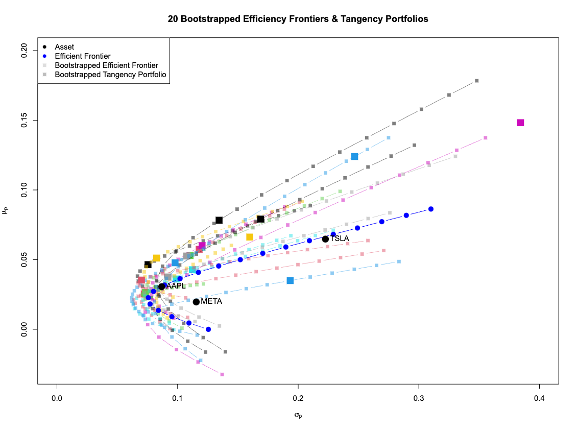
Twenty simulated Efficiency Frontiers and Tangency Portfolios

Our analysis showcased how small fluctuations when simulating the individual asset returns lead to large errors in the asset spread of the optimal Tangency Portfolio. Most simulations overestimated both the risk and return of the tangency portfolio. Including Rolling Analysis may give a better prediction for spreading investments.